[Information in italics is not crucial to a qualitative understanding of what's going on. It is just added in case you start thinking too deeply for the simple explanations.]

1) Why can't one use a powerful light microscope to see bonds?

2) Just HOW is structural information contained in diffracted X-rays?

a) A single pair of scattering points
b) An infinite row of evenly spaced scattering points
c) A row of evenly spaced pairs of scattering points
d) An hexagon of points ("benzene")
e) A pair of hexagons
f) A quartet of hexagons
g) A lattice of hexagons
h) Significance

3) What does Rosalind Franklin's x-ray photo show about b-DNA?

a) Start by understanding the lightbulb filament.
b) Base-Pair Stacking
c) Diameter
d) Double Helix - Major and Minor Grooves

4) What does the electron density in a molecule look like? Are there Lewis Shared Pairs?

a) How to plot 3D electron density
b) What do e-density maps say about molecules, atoms, and bonds?
c) Accurate Difference Density maps show bonds

5) Conclusions

Light is ELECTROMAGNETIC RADIATION. It consists of electric and magnetic fields that are oscillating perpendicular to the direction in which the light is travelling (and perpendicular to one another). For our present purposes we are interested in the electric field, since that is the main actor in pushing electrons around.

One can graph the oscillating electric field of light as a sine wave, where the vertical axis is the FIELD STRENGTH (+ or - means pointing one direction or the other, i.e. exerting a force on an electron in one directon or the other), and the horizontal axis can be either TIME or POSITION. That is, we can plot the change of the field with time at any given position (perhaps where a particular atom is), or we can plot the change of field with position along the direction of light propagation at some given time.

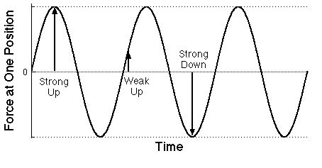
Graph of the force on an electron at some particular position as a function of time due to the electric field of a particular light wave. Of course the force on a proton would be just the opposite. One over the time difference between successive maxima is the frequency of the light.
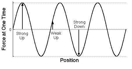
Graph of the force on electrons at some particular time as a function of the position of each electron measured along the direction that the light wave is moving. Note that only the labels have been changed from the plot above. The distance between successive maxima is the wavelength of the light. As for a water wave, there are two different ways of describing light with a wave-shaped plot.
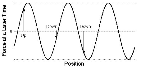
Graph of the force on the same electrons at a later time than shown in the previous plot as a function of the position of each electron position measured along the direction that the light wave is moving. The forces can change in both size and direction. As time goes by, the wave moves to the right, the direction of light propagation.

The electric field of light pushes charged particles of matter, and the accelerating charges create new light waves that move off in all directions, not just the direction in which the original light wave is moving. This is called SCATTERING. Of course the electrons, being more than 1000 times lighter than the lightest nucleus, are accelerated much more than the nuclei, so light is scattered predominantly by electrons.

Thus if a light beam hits stuff and gets scattered, your eye can detect light even though it is not in position to be struck by the incoming beam. Deflected light is the signal that there must have been electrons in the light path to do the scattering.

It is good to have a way of knowing that there are electrons in the light path, but we want to know more. We want to know where they are, how they are distributed, that is we want to know the STRUCTURE of the matter that is doing the scattering. In particular, we want to know if electrons are gathered around nuclei to form atoms and whether pairs of electrons concentrate between certain pairs of nuclei to constitute Lewis shared-pair bonds. This is related to the problem of RESOLUTION (how far apart two things have to be in order to tell that they are not a single piece).

One way to determine structure is to scan a VERY narrow beam back and forth, up and down across the sample and see where scattering originates. This "raster "scanning (as in TV, or SPM) is used in scanning electron microscopy and in an SPM technique called SNOM (Scanning Near-field Optical Microscopy); but beams can't be made narrow enough to resolve adjacent small molecules, let alone atoms. Is there an alternative to scanning for coding structural information into the scattered light? There must be, because our eyes don't work by raster scanning.

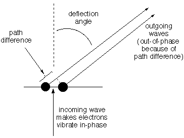
Structural information is coded into an INTERFERENCE PATTERN. Imagine two electrons side-by-side in the path of the same incoming wave so they are made to vibrate up and down in phase with one another. Consider the oscillating electric field that hits a detector at a very great distance [so distant that there is no significant difference between the two electrons in the angle by which the beam is deflected to hit a certain spot on the detector]. The total field is the sum of the two scattered fields, and because the path for one is longer than for the other, depending on the angle, the two waves will have different phase at any given time, one may be pushing up when the other is pushing down, for example. If the path difference is exactly one (or two, or three...) waves, the fields will reinforce one another to give a field twice as strong as that from one electron. If the difference is half a wave, they will cancel. Thus as the deflection angle increases from zero the amplitude detected for the scattered wave will decrease, then increase, then decrease, etc. How rapidly the amplitude of the composite scattered beam changes with increasing angle depends on the distance between the electrons and the wavelength of the light. Decoding this information about distance is the job of the lens of the microscope (or the lens and retina of your eye). We need not be concerned with the decoding, just with whether the structural information is present to be decoded.

[The "wave machine" shown in class illustrated how such interference arises. To be picky I should note that we're ignoring certain pathological situations where electrons in different kinds of atoms may not vibrate precisely in phase with one another even when they are being struck at the same time by the same wave. This situation is called anomalous dispersion, and can be quite useful.]

If the wavelength is much greater than the distance between the electrons, there can be no significant difference in phase for any scattering angle, and thus no clue in the scattered light that there are two separate electrons. We can only resolve objects whose separation is comparable to, or larger than, the light wavelength. [Note that the greatest phase difference occurs for light scattered at 90° from the incoming ray. Thus to get maximum resolution from light of a given wavelength one must collect scattered light up to a wide angle. This is why the objective lens of a high-power microscope must get very close to the object in view.]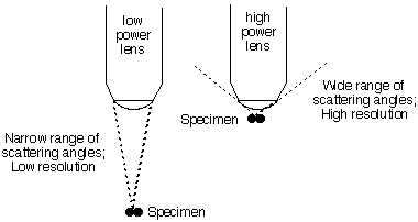

The shortest visible wavelength is >400 nm = 4000 Å, ~ 2700 times the C-C bond distance. So forget using light microscopes to resolve adjacent atoms within molecules or even adjacent molecules of reasonable size.

If we want to resolve atoms, we must use waves that are about 1.5 Å (0.15 nm) long. This means X-rays, but there is no good lens for focussing x-rays, so we must use a computer to decode the structural information from the interference pattern collected over a wide range of angles.

[High-kinetic-energy electrons also behave as waves with short wavelength, and there are electric "lenses" for them. They can be used for transmission electron microscopy (TEM), but they are much less generally useful than x-rays, because electrons are so strongly scattered that they can't go through air or through more than a few molecular layers of a sample.]

2) Just HOW is structural information contained in diffracted X-rays?

It is easy to appreciate that, if the wavelength of the light is short enough (x-rays), scattered light contains information about how electrons are distributed in a sample. [A good analogy is a water wave which encounters the pilings in a pier and generates a complex pattern of reflected waves that depends on how the pilings were arranged.]

The problem is how to decode the information.

Nowadays sophisticated computer programs can do the decoding pretty easily for crystals of even rather large molecules - most recently and dramatically (and at Yale) the ribosome with hundreds of thousands of atoms. For most people these programs are just black boxes. It is rewarding to think a little about how the information is contained in the scattered X-rays. This is why we used the He/Ne laser (wavelength 632.8 nm) in the lecture demonstration.

[First we think of scattering within a single plane, as visualized with the "wave machine". The first slides used in the lecture demonstration consisted of vertical lines which, viewed from above look like the "points" discussed below. I give this technical information for the sake of honesty - you may stick with 2 dimensions and think of points instead of lines to get the idea. It is cute that in 3-D, just as a set of parallel lines on the slide give a row of dots on the screen, a row of dots on the slide gives a set of parallel lines on the screen.]

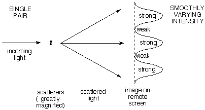
a) A single pair of scattering points (e.g. electrons) gives an intensity distribution that varies smoothly with increasing scattering angle from maximum (straight ahead) to minimum to maximum. The angular distance between maxima (together with the wavelength) tells how far apart the points are. Note the RECIPROCAL relationship: the closer the points are together, the larger the angular difference between scattered maxima. The first deflected maximum comes when the wavelets from the two scatterers differ by one wavelength, the second when they differ by two, and so on.

You are probably familiar with this case already as the "two-slit" experiment in which a plane wave of light travelling left to right passes through two slits viewed end-on 1/4 and 3/4 up the left side of the diagram. The resulting waves interfere (add to one another) to give at some instant in time the pattern shown. The light areas are peaks and the dark areas are troughs. Note that as the light moves far to the right the patterns coalesce into a set of rays fanning out from a point between the slits, and separated by gray areas of zero electric field. This gives the smoothly varying intensity shown on the remote screen in the diagram above. If you'd like to see an animation of these interfering waves, click for the applet at the Physics 2000 website.

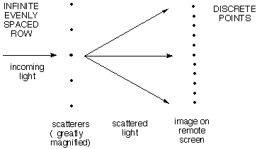
b) An infinite row of evenly spaced scattering points gives a row of discrete scattered spots. If the angle is chosen so that the waves scattered from the first two points differ by exactly one wavelength, the wave from the third will differ from that from the first by two wavelengths, etc. So all the waves will be effectively in phase to give very strong constructive interference. If the angle is changed just a little bit so that the first two waves are not exactly one wavelength different, the next will differ by twice as much, and so on, so that ultimately cancellation will set in.

For example, if waves from the the first two scatterers differed in phase by only 1% of a wavelength, the 50th would differ from the first by half a wavelength, and they would cancel. The 51st would cancel the 2nd, and so on. So there is a lot of blank space between successive maxima. As above, the angular distance between maxima (together with the wavelength) tells how far apart adjacent points are, and the relationship is reciprocal, large spacing of scatterers means close spacing of spots in the image.

The problem assigned in class was to determine the spacing between the rows on the slide that would give diffraction maxima separated by 10.8 cm on a screen at a distance of 10.6 m when the wavelength is 633 nm. (the answer is about 65 μm). Doing the geometry will confirm your understanding of the source of interference. Consider whether the observed points in the diffraction pattern should be spaced exactly evenly.

c) More interesting is a row of evenly spaced PAIRS of scattering points, where the pairs are closer together than the repeat distance between pairs. Here the pattern is the row of closely-spaced dots expected from (b) for the large repeat distance between pairs (remember the reciprocal relationship between spacing and angle), but the intensities vary slowly as expected from (a) for the smooth variation due to the members of a single closely-spaced pair.

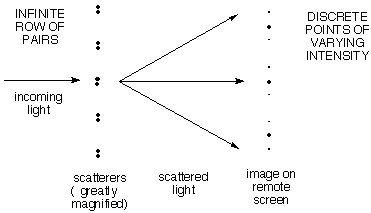
Here's how to think about this:

The pattern which is to be repeated generates a smooth variation of scattered intensity that tells about the structure of the pattern.

Here the pattern is a pair of dots. We know above that any pair of dots with this spacing will scatter with a smooth variation in intensity as shown in (a) above. Since all of the pairs have the same spacing, they will all scatter with the same angular dependence. Now all we have to worry about is how the scattering from one pair interferes with that from the others.

The fact of the regular repetition allows one to observe this scattered intensity only at the discrete positions allowed by the repeat distance. [Importantly, the net scattered intensity is unchanged. It is as if the intensity of the diffuse pattern is gathered into the spots. This makes the spots easy to measure.]

This is like viewing the smooth distribution due to the pattern through little holes whose spacing is determined by (and reciprocal to) the row repeat, but the intensity is correspondingly amplified to preserve the total amount of scattered light.

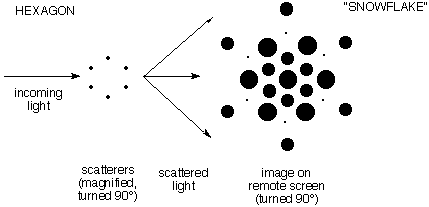
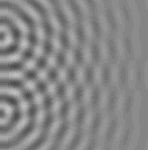
d) The second demonstration showed scattering in three dimensions. It involved a hexagon of points ("benzene"). A single set of six points generated a smoothly varying "snowflake" pattern of scattered intensity. The following illustration gives an idea of the diffraction pattern, but fails to shows how smoothly it varies. (Note: In this schematic illustration the pictures of the scatterers and the diffraction image are turned 90° so you can see them. Actually they lie on planes perpendicular to the ray of incoming light.) Click here to see the Laser Demonstration

[In order to get enough intensity to be visible the slide actually had an enormous number of hexagons, all oriented the same way but randomly placed. Randomly placed patterns give the same diffraction as single patterns, but more intense. This contrasts with a lattice of regularly placed patterns, which focuses the scattering into discrete points, as described in e-g.]

e) When the pattern contained pairs of "benzenes" the diffraction showed the same snowflake pattern but with intensity varying along the direction in which the pairs are displaced. Click here to see the Laser Demonstration
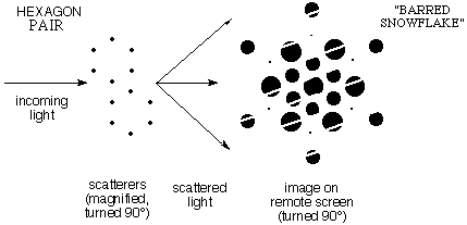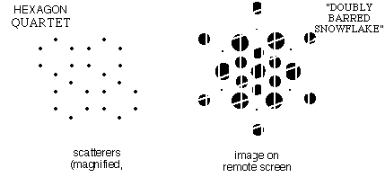
f) When the pattern contained quartets of "benzenes" at the corners of a parallelogram, the same snowflake pattern was modulated in intensity in two directions. Click here to see the Laser Demonstration

g) When all of the "benzenes" in the slide fell on a regular lattice with standard row and column spacing, the diffraction pattern showed the intensity distribution of the original snowflake but viewed only on the two dimensional lattice of points allowed by the regular spacings in rows and columns. This is the 2-dimensional analogue of (c) above. It is as if the snowflake were being viewed through the holes in a piece of pegboard.

h) Significance:

The LOCAL ELECTRON DISTRIBUTION (molecular structure) is coded in the INTENSITY of the spots (in this case, the underlying continuous snowflake pattern).

The SPACING OF THE ROWS AND COLUMNS (crystal lattice) is coded in the ARRANGEMENT of the spots (the "pegboard" holes through which the snowflake is seen).

X-ray diffraction is usually measured with single crystals. The crystal serves two purposes:

First, it orients all of the molecules in the same way, so the "snowflakes" reinforce.

Second, it concentrates all of the scattered light into a small number of points which are bright enough to observe easily.

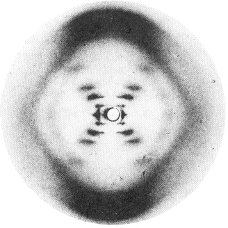
3) What does Rosalind Franklin's x-ray photo show about b-DNA?

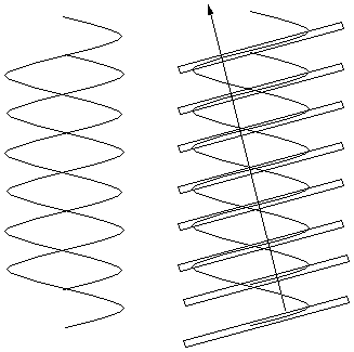
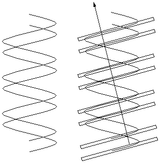
The diffraction of He/Ne red light by a slightly stretched filament from a broken lightbulb shows an "X" with spots along each leg (see below). This dotted "X" bears a strong resemblance to Franklin's photo (right) of DNA fibers in which long molecules were oriented more or less vertically by stretching. Since neither the filament nor the DNA is crystalline, both show the rather diffuse pattern from an individual object (like a pair - or hexagon - of dots) rather than the set of sharp spots characteristic of an infinite regular lattice of such objects. Of course there is a certain degree of repetition within the helix itself, which gives rise to the features that are discussed below. These helices are great examples of how molecular structural information is present in the scattering pattern. For example, the regular repetition from turn to turn along the helix axis constitutes a repeating vertical pattern that gives rise to horizontal bars, as in 2c or 2e above.

a) Start by understanding the lightbulb filament.

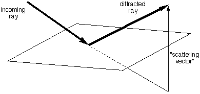
We need the following rule: All electrons on the same plane perpendicular to the scattering vector (the change in light direction, which bisects the incoming and outgoing rays, see figure) scatter with the same phase. [This is in fact how a mirror works - all the silver atoms scatter light in phase when the incoming and outgoing beam angles are the same.] For purposes of calculating the scattered intensity, all the electron density in such a plane could all be considered as concentrated at any single point on the plane perpendicular to the scattering vector. THIS IS A VERY NEAT TRICK. [It is easy to prove this rule geometrically by showing that all the path lengths (sum of incoming and outgoing) are the same]

So we can look for planes in the sample that have a lot of electron density and think about the light that is scattered (or "reflected") from them. For a vertical helix (right) there is a lot of electron density on the slanted planes shown (middle and far right), and not much on any given parallel plane between them. Thus the indicated scattering vectors should be imporant. That is, some of the light going perpendicularly into the page should be deflected up to the left (and down to the right) by the "planes" highlighted in the center figure. Some should also be deflected down to the left (and up to the right) by the "planes" highlighted in the right figure. These are the directions of the arms of the "X".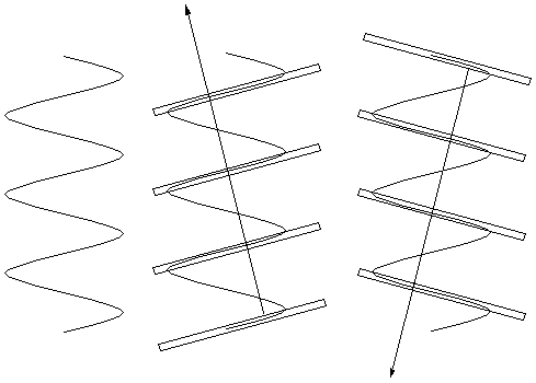

[Actually the helix must be slightly tilted to bring these particular planes into reflection position. This may be taken care of by rocking the sample a bit during exposure of the film, or, as in the Franklin case, by the fact that different molecules in the fiber have slightly different orientations so that many have the desired orientation of slight tilt in any given direction. Even without the axis tilting, there will be an analogous set of planes slightly further along the helix (and a few degrees around to the right) that will be tilted into the correct position. This is a fine point - don't waste time on this if you don't see it right away. There are more important things to think about.]

For scattering in the indicated directions the e-density on the planes could be thought of as concentrated at the points where the arrow intersects the planes. That is, there is scattering as if from a row of dots, that we know would reinforce at a given succession of angles (as in 2b above). There is very little electron density on the interleaving planes, where it would have to be to cancel these reinforcing waves.

Thus the "X" of dots in Franklin's photo shows that DNA is a helix, and the angle of the "X" shows how tightly it is wound (think about this).

b) Base-Pair Stacking

Successive units of the DNA chain are spaced at a regular distance along the axis of the helix. For example, one can see planes that contain practically all of the carbon and nitrogen atoms of the "bases" in stacked planes perpendicular to the axis. These planes are much closer together than the "helix planes" illustrated above so they should reinforce for scattering at a much higher angle. This gives rise to the very dark spots at the top and bottom of the Franklin picture and shows that the stacking distance is 3.4 Å (the thickness of an aromatic ring).

c) Diameter Much of the electron density of DNA is in the phosphorous and oxygen atoms on the helical chain. Thus lots of the electron density lies on the periphery of a cylinder. The illustration to the right shows that planes that are nearly tangent to the cylinder contain lots more electron density than those halfway between them (because the center is not so dense in electrons. This gives lateral scattering that measures the 20 Å diameter of the helix (the spots look like triangles in Franklin's photo).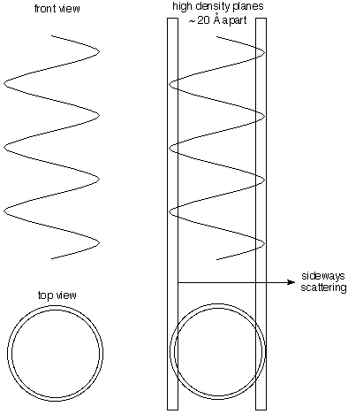

d) Double Helix - Major and Minor Grooves

Other things being equal, spots get less intense as they move to higher scattering angle. This is observed as one moves out along the arms of the "X" from the lightbulb filament scattering.

[This is because the atoms have finite size, so that scattering from one portion of an atom can interfere with that from another portion of the same atom.  This becomes more important as the relevant planes get closer together for "high-angle" scattering.]

Things are different for DNA. As one moves out from the center the 1st spot is rather weak, the 2nd and 3rd are strong, the 4th is too weak to see, and the 5th is strong enough to see clearly - much stronger than the fourth. What a queer sequence of intensities!

[Incidentally, the undeflected beam would be so strong as to wash out everything else - therefore a lead cup is put in its path to intercept it, so there is no spot in the center of the photograph.]

The intensities show that DNA is a double helix with a major and a minor groove Had the structure involved an evenly spaced double helix (as shown right) the spots on the "X" would be twice as far apart (i.e. every other spot from the single helix would be missing), because the slanted planes of electron density would be twice as close together. Another way of saying the same thing is the following: For a scattering angle where waves from successive planes in the same helix differ by an odd number of cycles (and thus reinforce one another), those from the other helix differ from them by a half-integral number of cycles and cancel the waves from the first helix. When reflections from successive planes of a single helix differ by an even number of light cycles, reflections from planes of the other helix differ from them by an integral number of cycles and reinforce.

But what if the helices are offset from even spacing to give major and minor grooves as shown to the right? The pattern of planes is like that of the spots in example 2c above - a widely spaced row of closely spaced pairs of scatterers. The resulting diffraction pattern would also be the same - a row of points spaced as for the row (single helix) spacing, but with modulated intensities (weak, strong, strong, very weak, intermediate) that can be used to measure the amount of offset between the two helices. This is exactly what the Franklin photograph shows.

4) What does the electron density in a molecule look like? Are there Lewis Pairs?

a) How do you visualize three dimensional plots of electron density?

Electron density is a function of three variables - x, y, and z positions. How can you plot it?

On a 2-dimensional sheet of paper it is convenient to plot two things against one another (two variables - independent and dependent). It is harder to plot a function of two variables, e.g. altitude (or temperature) as a function of latitude and longitude. With color or a gray scale it is possible to plot such a function of two variables. Another convention is to use a contour plot where lines connect two-dimensional locations of a given value. You should be familiar with such plots of isotherms (regions of the same temperature) and with topographic maps showing a mountain as a series of nested curves.(click here for a brief exercise on 3D plots)

Plotting a function of three variables is much more difficult. One way would be to take a big block of clear gelatin and use an hypodermic syringe with dye to inject more or less color in regions of certain electron density. One could generate an image of such an object using 3-D computer graphics (this is precisely what Dean Dauger did to represent the electron density in hydrogen-like atomic orbitals in his program Atom in a Box, which we'll be using soon). A practical scheme for presentation on paper is to make a well-chosen cut through 3-D space to define a particular plane of interest (for example a plane containing the atomic nuclei of a planar molecule) and then use a contour plot to show electron density on that single plane. One could make a lot a parallel planar cuts and show a bunch of such contour graphs. No one said it would be easy. (here is an example of such a planar map)

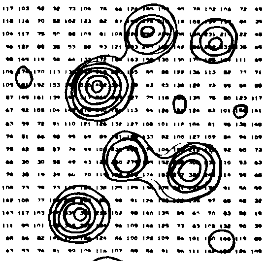
The figure to the right shows contours on part of an arbitrary slice through an e-density "map" from an X-ray study of Rubofusarin. In the old days numbers giving the e-density were typed on a page at the appropriate x,y positions by a computer and the crystallographer then connected locations of the same value with a pen to generate contours. This was about 40 years ago - before it was easy and cheap to make computers draw solid curves. There were no laser or ink jet printers or graphic (or color) terminals. Electric typewriters or close relatives were the common output devices. Imagine! From examining the numbers it looks to me as though they were contouring at values of 150, 200, 250, 300, 350, 400 (in arbitrary units, not e/Å3). (from Stout and Jensen "X-ray Structure Determination" 1968)

Not all of the atoms fell on the slice plotted above. Fortunately the molecule of Rubofusarin is nearly planar, so the crystallographer could calculate an analogous sheet of numbers for a different slice chosen to contain most of the molecule's atoms. He then traced a similar set of contours on an overlaid sheet of plain paper to give the figure shown to the right. Here he drew contours at intervals of 1 e/Å3.

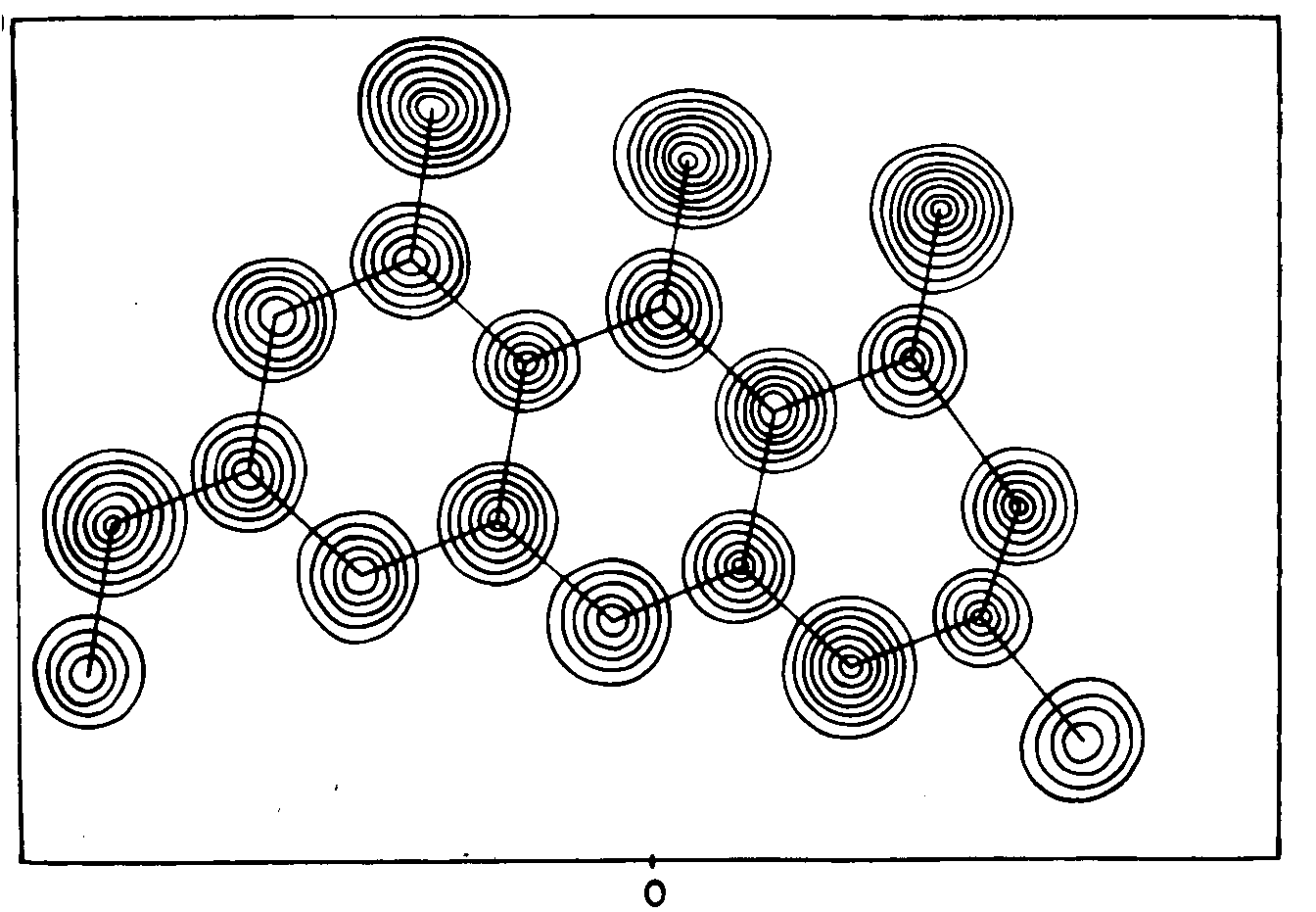Correspondence of the spheres of high electron density with the non-hydrogen atoms in the formula of Rubofusarin is obvious.

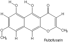
Rubofusarin has the advantage of being nearly planar, so that a single planar slice can give a good idea of the electron density of almost all of its atoms. In a non-planar molecule one must choose different slices to show features of the electron density with a two-dimensional contour map. One approach, used in the 1940s in connection with determination of the structure of the potassium salt of penicillin by Dorothy Crowfoot (later Hodgkin) at Oxford, is to draw contour maps for a set of sequential, parallel slices on transparent sheets and stack them up to give a three-dimensional contour map, actually a sort of four-dimensional graph! [KPenicillin illustration]

b) What do e-density maps say about molecules, atoms, and bonds?

There is a lot of information in this e-density map.

Perhaps the most important is that this organic molecule looks like a collection of spherical atoms with electron density increasing toward the nucleus of each. There is certainly no "double dot" of electron density between the atoms. In fact the spheres don't even look distorted. There is no evidence from this plot to support Lewis's idea that bonds consist of shared electron pairs!

Note that electron densities identify the atoms:

hydrogens have too little electron density to be visible in this map (less that 1 e/ų)
only oxygen atoms achieve electron density greater than 7 e/ų (seven contour lines).

The nuclei don't appear directly in the map, since they are too heavy to scatter x-rays significantly, but one can guess that they are located where the e-density is highest at the center of each sphere. [This inference can be confirmed by experiments involving neutron scattering - neutrons are scattered by nuclei and thus can reveal their position directly.]

The bond lengths show what kind of bond is involved:

Such e-density maps confirm the reality of molecules and atoms but not of the Lewis shared-pair bonds.

c) Accurate Difference Density maps show that electrons DO shift (a little) to make bonds.

Of course one can wonder whether the apparently spherical electron density distributions that look so much like isolated atoms might be at least a little bit distorted. The most sensitive way to check this is with a "charge-density difference map". Instead of plotting the total electron density, one plots the difference in density between what is observed in very accurate experiments and what would be expected for an analogous collection of perfectly spherical, undistorted atoms. If there is no distortion upon forming bonds, the difference density should be zero everywhere, but if electron density shifts a little, there will be positive regions where density accumulates and negative regions where it is depleted.

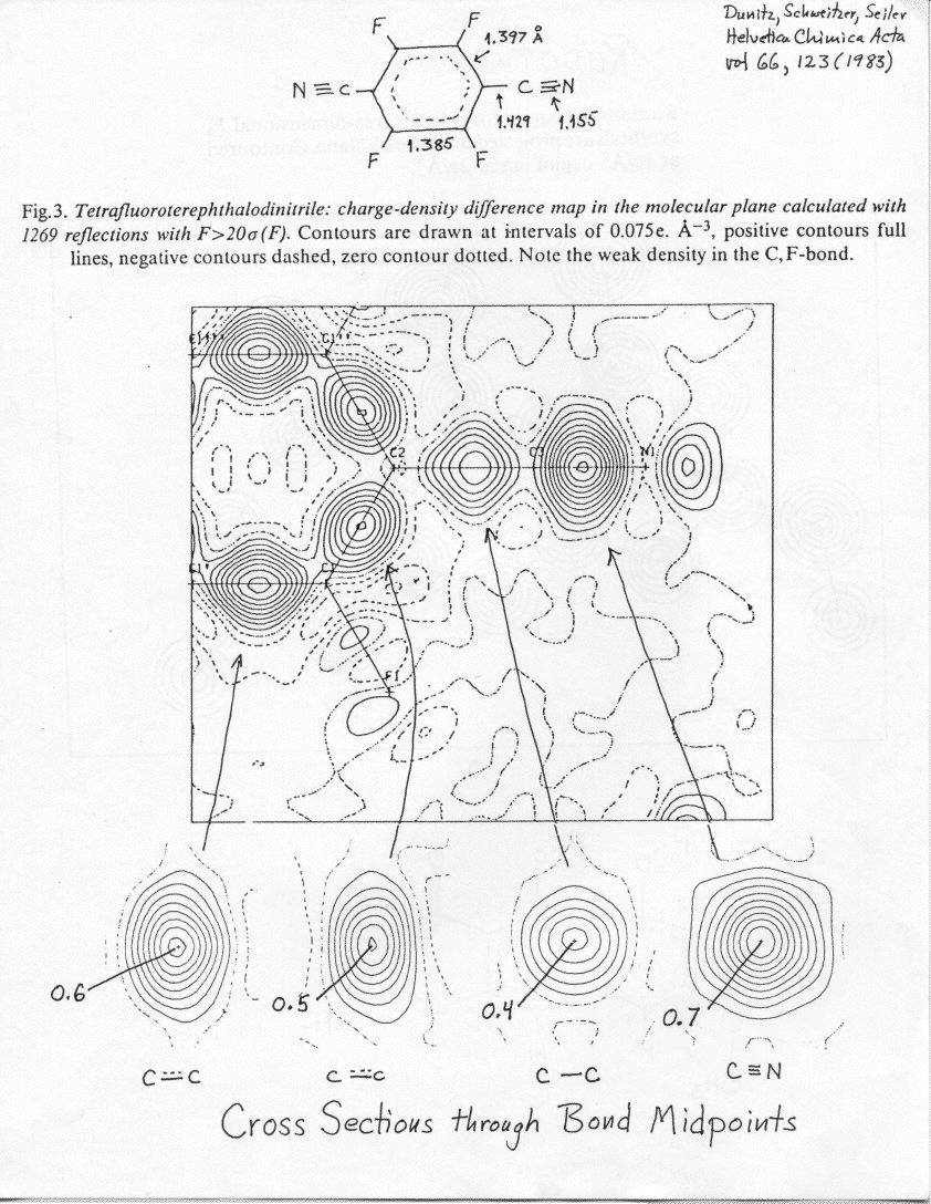
One lecture illustration showed such a difference density map for a molecule with single C-C bonds, aromatic C-C bonds, CN triple bonds, and C-F single bonds. Solid contours show where electron density increased upon forming bonds, and dashed (negative) contours show where it was depleted. Notice that the amount of density shifted is very modest - the contour level in the difference map is only 0.075 e/ų, less than one tenth of the 1 e/ų interval used in contouring the total e-density map above. Even if the triple bond the maximum increase in e-density between the nuclei is only 0.7 e/ų, less that 10% of the density near an oxygen nucleus. [Tetrafluorodinitrile illustration; see Lecture 6]

Lewis might have been gratified to see that, upon forming the molecule, e-density accumulates between the atoms in "bonds", and in an unshared pair on the nitrogen atom. [Lewis had died 20 years before experiments of sufficient accuracy were possible.] It is also satisfying to see that the greatest accumulation of e-density is in the triple bond, followed by the "resonant" aromatic "one-and-a-half" bonds, and the single bonds. [The much more modest accumulation in the C-F bonds is surprising and requires some mental gymnastics to rationalize. (see interview with J. D. Dunitz)]

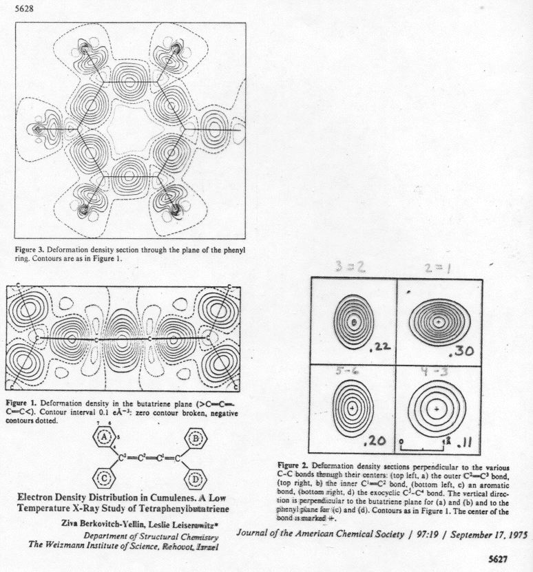
Perhaps even more striking is the cross sections of the bonds. The single and triple bonds have circular cross sections, while the aromatic bonds have oval cross sections consistent with the contribution from both sigma and pi bonds (which we will discuss a lot more later). [Cumulene overhead, see Lecture 6; see interview with L. Leiserowitz] [Cyclopropane illustration, see Lecture 7]

5) Conclusions

So, using "x-ray vision", we can see experimentally that molecules and atoms are real, and that bonding is associated with (modest) accumulation of electrons between the bonded atoms.

Here is the answer to "How do you know?" - not because some teacher or book told us there are atoms and bonds, but because it seems plausible that previous scientists accurately reported x-ray experiments of which we understand the significance. If we were skeptical, we could repeat the experiments and see for ourselves.

Our next task is to understand WHY the electrons gather into bonds and what properties bonds should have (length, angles, strength, reactivity), and more fundamentally what is special about octets, why there are electron shells, etc.